LSTM vs Tolkien
«««< HEAD This notebook is greatly inspired by this notebook by G. Negrini. Please check out his website as he makes really good content. In the orginal notebook, he used the Keras library while this approach is based on duo Jax + Haiku from DeepMind. Here we will try to recognize between drug names and Tolkien characters using a simple LSTM model which surprisingly isn’t as easy as one can think. If you want to challenge yourself here is a popular website with a great quiz. ======= This notebook is greatly inspired by this notebook by G. Negrini. Please check out his website as he make really good content. In original notebook he used Keras library while this approach is based on duo Jax + Haiku from DeepMind. Here we will try to recognize between drug names and Tolkien characters using simple LSTM model which surprisingly isn’t as easy as one can think. If you want to challenge yourself here is popular website with great quiz.
93b45c0d86afd75ba404fcba7c1e72635d199e1c
import jax
import haiku as hk
import pandas as pd
import matplotlib.pyplot as plt
import seaborn as sns
from jax import numpy as jnp
import numpy as np
from sklearn.model_selection import train_test_split
from haiku import nets as nn
import optax
from tqdm.notebook import tqdm
from typing import Optional
sns.set_theme()
np.random.seed(42)
Data
Fortunately following the original notebook we can find a great database with tolkien names on www.behindthename.com.
raw_tolkien_chars = pd.read_html('https://www.behindthename.com/namesakes/list/tolkien/name')
raw_tolkien_chars[2].iloc[200:210,:]
| Name | Gender | Details | Total | |
|---|---|---|---|---|
| 200 | Damrod | m | 1 character | 1 |
| 201 | Déagol | m | 1 character | 1 |
| 202 | Denethor | m | 3 characters | 3 |
| 203 | Déor | m | 1 character | 1 |
| 204 | Déorwine | m | 1 character | 1 |
| 205 | Derufin | m | 1 character | 1 |
| 206 | Dervorin | m | 1 character | 1 |
| 207 | Diamond | f | 1 character | 1 |
| 208 | Dina | f | 1 character | 1 |
| 209 | Dinodas | m | 1 character | 1 |
We can see not only names contain non-ASCII characters so we need to preprocess our data. We will lower all characters and replace every character to an ASCII base.
tolkien=np.array(list(map(lambda x:x
                          .replace("-","")
                          .encode("ascii","ignore")
                          .lower(),raw_tolkien_chars[2]["Name"].values)))
Following original notebook we will use medication guide from US Food & Drug Administration and use similar preprocessing as before.
raw_medication_guide = pd.read_csv('Medication Guides.csv')
id=np.random.randint(0,len(raw_medication_guide["Drug Name"].unique()),size=10)
raw_medication_guide["Drug Name"].unique()[id]
array(['Bydureon Pen', 'Optimark in Plastic Container', 'Hulio',
       'Caprelsa', 'Avinza', 'Voltaren', 'Adderall 15', 'Technivie',
       'Cipro XR', 'Plavix'], dtype=object)
drugs=np.unique(np.array(list(map(lambda x:x.split()[0]
                                  .replace("-","").replace(".","")
                                  .encode("ascii","ignore")
                                  .lower(),raw_medication_guide["Drug Name"]
                                  .drop_duplicates()))))
print(len(tolkien),len(drugs))
746 674
After preprocessing we are left with \(746\) unique Tolkien names and \(674\) unique drug names so we have rather balanced dataset.
There are few approaches we can use to preprocess data. One can replace each character by corresponding integer number which should be further preprocessed either by one-hot encoding or embedding into high-dimensional space. Because we have only 26 characters we will follow original approach and one-hot encode our values.
def tokenize(string):
    return jnp.array(list(map(lambda x:x-ord("a"),string)))
X_train=np.concatenate((tolkien,drugs))
Y_train=jnp.concatenate((jnp.zeros(tolkien.shape[0]),jnp.ones(drugs.shape[0])))
X_train=list(map(tokenize,X_train))
Finally we split train and validation data using sklearn with ratio \(0.8\).
X_train,X_val,Y_train,Y_val=train_test_split(X_train,Y_train,train_size=0.8)
Model
Now we implement simple LSTM model with Haiku. We have one layer of LSTM with dimension we specify followed by one dense layer with dropout. Instead of simple classification head or multiclassification task we will use two binary classification heads for each class. We will also model logits during training as we will use the fact that binary cross-entropy have simple when modeling logits instead of probabilities. Instead of using hk.dynamic_unroll as typically we will use hk.scan which is thin wrapper around jax.lax.scan with additional parameter unroll allowing to choose option in between static unroll and full dynamic unroll. Between layers we use GeLU activation instead of ReLU.
def reverse(t): #we need to reverse our sequence as scan needs function with signature F(carry,x)
    return t[1],t[0]

class Model_LSTM(hk.Module):
    def __init__(self,size: int
                 ,p: float
                 ,unroll: Optional[int]=1
                ) -> None:
        super().__init__()
        self.size = size
        self.p = p
        self.unroll = unroll
        self.lstm = hk.LSTM(self.size)
        self.linear = hk.Linear(2)
        self.drop = hk.dropout
    def __call__(self,x:jnp.array,key,testing:bool) -> jnp.array:
        state = self.lstm.initial_state(x.shape[1])
        state,x = hk.scan(lambda a,b:reverse(self.lstm(b,a)),state,x,unroll=self.unroll)
        x_final = jax.nn.gelu(x[-1,:,:])
        x = self.linear(x_final)
        if not testing:
            x = self.drop(key,self.p,x)
            return x
        else:
            return jax.nn.sigmoid(x)
Now let’s specify model parameters and write down the training loop we will use to train our model. We use LSTM with dimensionality \(8\) and dropout \(0.05\).
lstm=hk.transform(lambda x,key,testing=False: Model_LSTM(8,0.05)(x,key,testing))
key=hk.PRNGSequence(42)
params=lstm.init(next(key),x=jnp.ones([4,1,26]),key=next(key)) #dummy varible to specifiy dimensionality
def train(lstm,num,params,X_train,Y_train,batch_size,save=2):
    opt=optax.adam(learning_rate=2e-4)
    opt_state=opt.init(params)
    seq=hk.PRNGSequence(42)
    @jax.jit
    def loss_binary(params,X,Y,key):
        key1,key2=jax.random.split(key)
        Y_pred=lstm.apply(rng=key1,params=params,x=X,key=key2)
        return optax.sigmoid_binary_cross_entropy(Y_pred,Y).sum()

    @jax.jit
    def update(opt_state, params, X, Y,key):
        l, grads = jax.value_and_grad(loss_binary)(params, X, Y,key)
        updates, opt_state = opt.update(grads, opt_state, params)
        params = optax.apply_updates(params, updates)
        return l, params, opt_state

    @jax.jit
    def acc_t(params,X,Y,key):
        l=lstm.apply(rng=key,params=params,x=X,key=key,testing=True)
        Y_pred=jnp.argmax(l,axis=1).reshape(1,1)
        return jnp.sum(Y_pred==Y)
    loss_arr=np.zeros(num//save)
    acc_arr=np.zeros(num//save)
    for N in (range(num)):
        idx=np.random.permutation(len(X_train))
        loss=0/len(X_train)
        for id,i in enumerate(idx):
            X=jax.nn.one_hot(X_train[id],num_classes=26).reshape(len(X_train[id]),1,26)
            Y=jax.nn.one_hot(Y_train[id],num_classes=2)
            l,params,opt_state=update(opt_state,params,X,Y,next(seq))
            loss+=l
        if N%save==0:
            acc=0
            for X,Y in zip(X_val,Y_val):
                X=jax.nn.one_hot(X,num_classes=26).reshape(len(X),1,26)
                acc+=acc_t(params,X,Y,next(seq))
            acc/=len(X_val)
            print('epoche:{0:} ,loss: {1:.2f}, accuracy: {2:.3f}'.format(N,loss,acc))
            acc_arr[N//save]=acc
            loss_arr[N//save]=loss
    return params,acc_arr,loss_arr
key=hk.PRNGSequence(42)
Num=50
save=2
params=lstm.init(next(key),x=jnp.ones([4,1,26]),key=next(key))
params,acc_arr,loss_arr=train(lstm,Num,params,X_train,Y_train,1,save=save)
epoche:0 ,loss: 1571.16, accuracy: 0.602
epoche:2 ,loss: 1443.97, accuracy: 0.729
epoche:4 ,loss: 1248.24, accuracy: 0.746
epoche:6 ,loss: 1138.09, accuracy: 0.771
epoche:8 ,loss: 1053.81, accuracy: 0.789
epoche:10 ,loss: 998.06, accuracy: 0.799
epoche:12 ,loss: 944.48, accuracy: 0.813
epoche:14 ,loss: 911.60, accuracy: 0.806
epoche:16 ,loss: 899.01, accuracy: 0.810
epoche:18 ,loss: 887.94, accuracy: 0.824
epoche:20 ,loss: 867.32, accuracy: 0.820
epoche:22 ,loss: 845.32, accuracy: 0.827
epoche:24 ,loss: 839.61, accuracy: 0.831
epoche:26 ,loss: 821.87, accuracy: 0.827
epoche:28 ,loss: 816.82, accuracy: 0.831
epoche:30 ,loss: 806.93, accuracy: 0.827
epoche:32 ,loss: 801.71, accuracy: 0.827
epoche:34 ,loss: 790.72, accuracy: 0.827
epoche:36 ,loss: 782.85, accuracy: 0.820
epoche:38 ,loss: 778.10, accuracy: 0.827
epoche:40 ,loss: 756.51, accuracy: 0.838
epoche:42 ,loss: 745.02, accuracy: 0.835
epoche:44 ,loss: 754.22, accuracy: 0.831
epoche:46 ,loss: 746.22, accuracy: 0.827
epoche:48 ,loss: 731.05, accuracy: 0.827
Now it’s time to show what we have learned.
fig,[ax1,ax2]=plt.subplots(1,2,figsize=(10,5))
ax1.plot(np.arange(0,Num,save),loss_arr)
ax1.set_xlabel("epoche")
ax1.set_ylabel("loss")
ax2.plot(np.arange(0,Num,save),acc_arr)
ax2.set_xlabel("epoche")
ax2.set_ylabel("accuracy")
plt.suptitle("LSTM model")
plt.tight_layout()
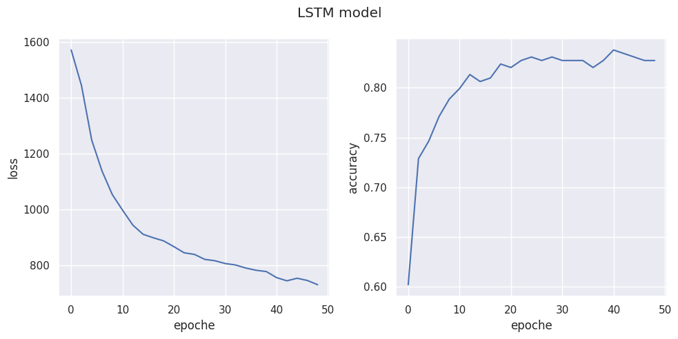
«««< HEAD We can see that after \(\sim 20\) epochs, we reach maximum accuracy despite decreasing loss as we probably hit the limit of our model but to be honest I think it’s really impressing behaviour as net outperforms me by far when it comes to ======= We can see that after \(\sim 20\) epochs we reach maximum accuracy despite decreasing loss as we probably hit limit of our model but to be honest I think it’s really impressing behaviour as net outperforms me by far when it comes to
93b45c0d86afd75ba404fcba7c1e72635d199e1c name recognition.
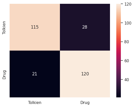
Now let’s investigate the confusion matrix for our validation set followed by the classification report.
from sklearn.metrics import confusion_matrix,classification_report
@jax.jit
def predict(X,key):
    key1,key2=jax.random.split(key)
    X=jax.nn.one_hot(X,num_classes=26).reshape(-1,1,26)
    return jnp.argmax(lstm.apply(x=X,rng=key2,key=key1,params=params),axis=1)
predictions=[]
for X in X_val:
    predictions.append(float(predict(X,next(key))))
matrix=confusion_matrix(Y_val,predictions)
sns.heatmap(matrix,xticklabels=["Tolkien","Drug"],yticklabels=["Tolkien","Drug"],annot=True,fmt="d")
<AxesSubplot: >
print(classification_report(Y_val, predictions, target_names=['Drug', 'Tolkien']))
              precision    recall  f1-score   support

        Drug       0.85      0.80      0.82       143
     Tolkien       0.81      0.85      0.83       141

    accuracy                           0.83       284
   macro avg       0.83      0.83      0.83       284
weighted avg       0.83      0.83      0.83       284
«««< HEAD We see that drug prediction has slightly better precision while Tolkien names have better recall. ======= We see that drugs prediction have slightly better precision while Tolkien names have better recall.
93b45c0d86afd75ba404fcba7c1e72635d199e1c